Understanding how a robot learns to pour tea using diffusion models
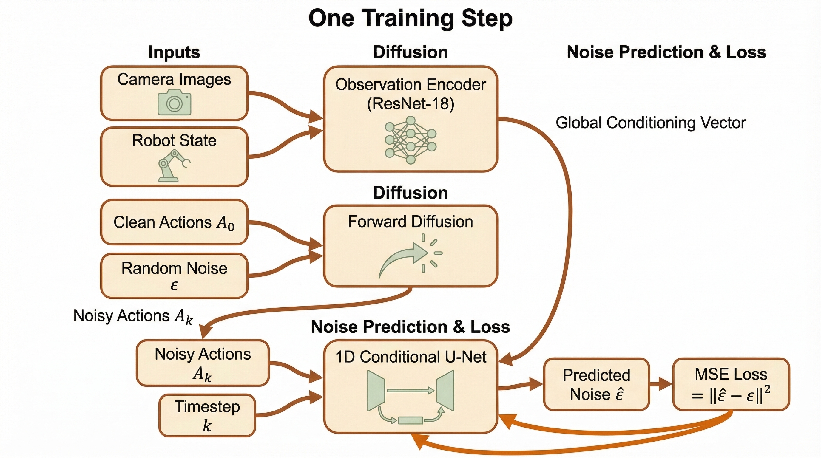
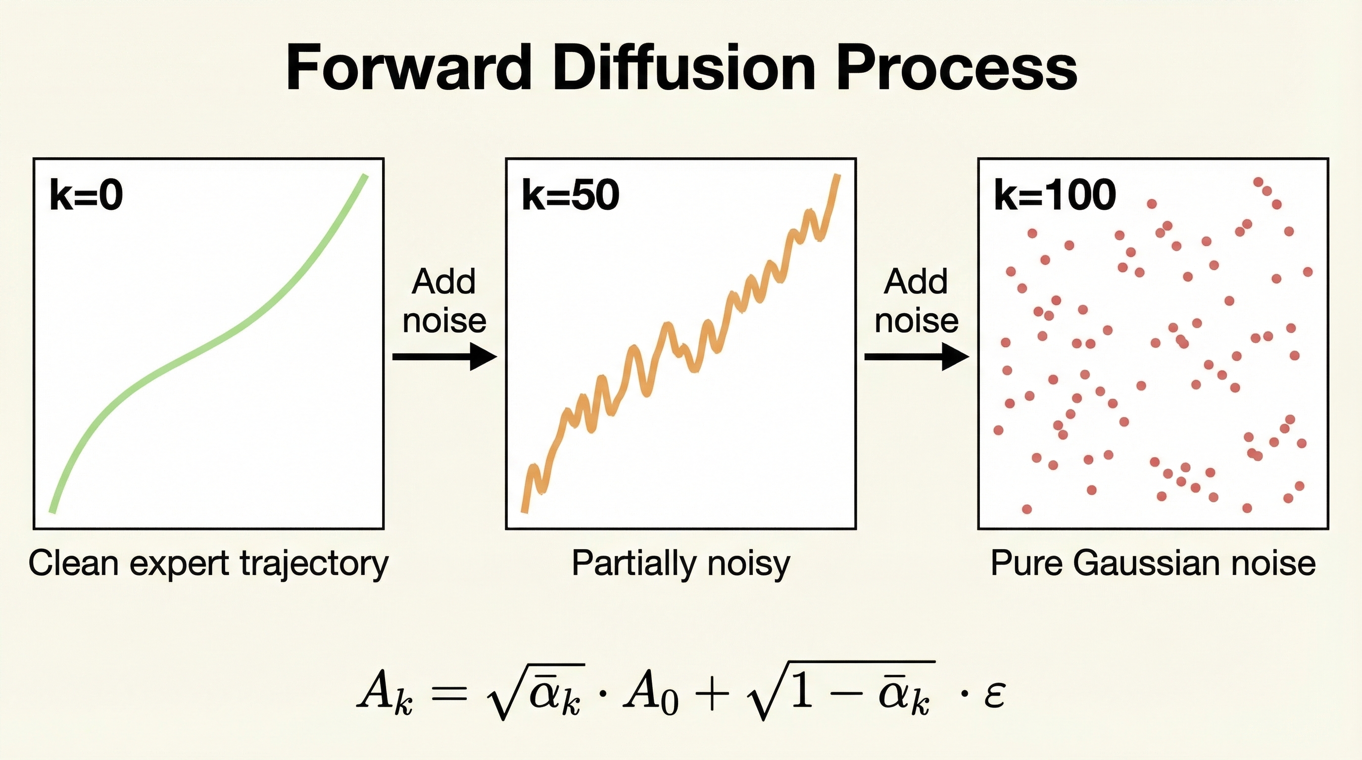
Diffusion Policy learns robot actions by treating the action trajectory (a sequence of future robot movements) as something that can be gradually corrupted with noise and then recovered by a neural network.
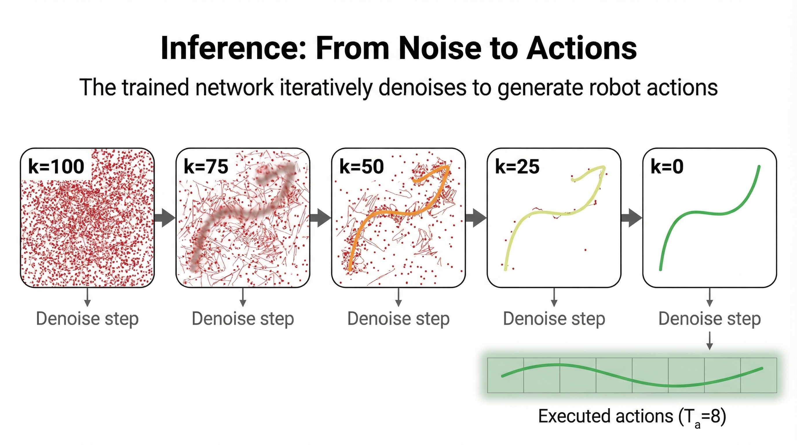
During training, we add noise to expert action trajectories and train a neural network to predict that noise. During inference, we start from pure noise and iteratively denoise to generate actions.
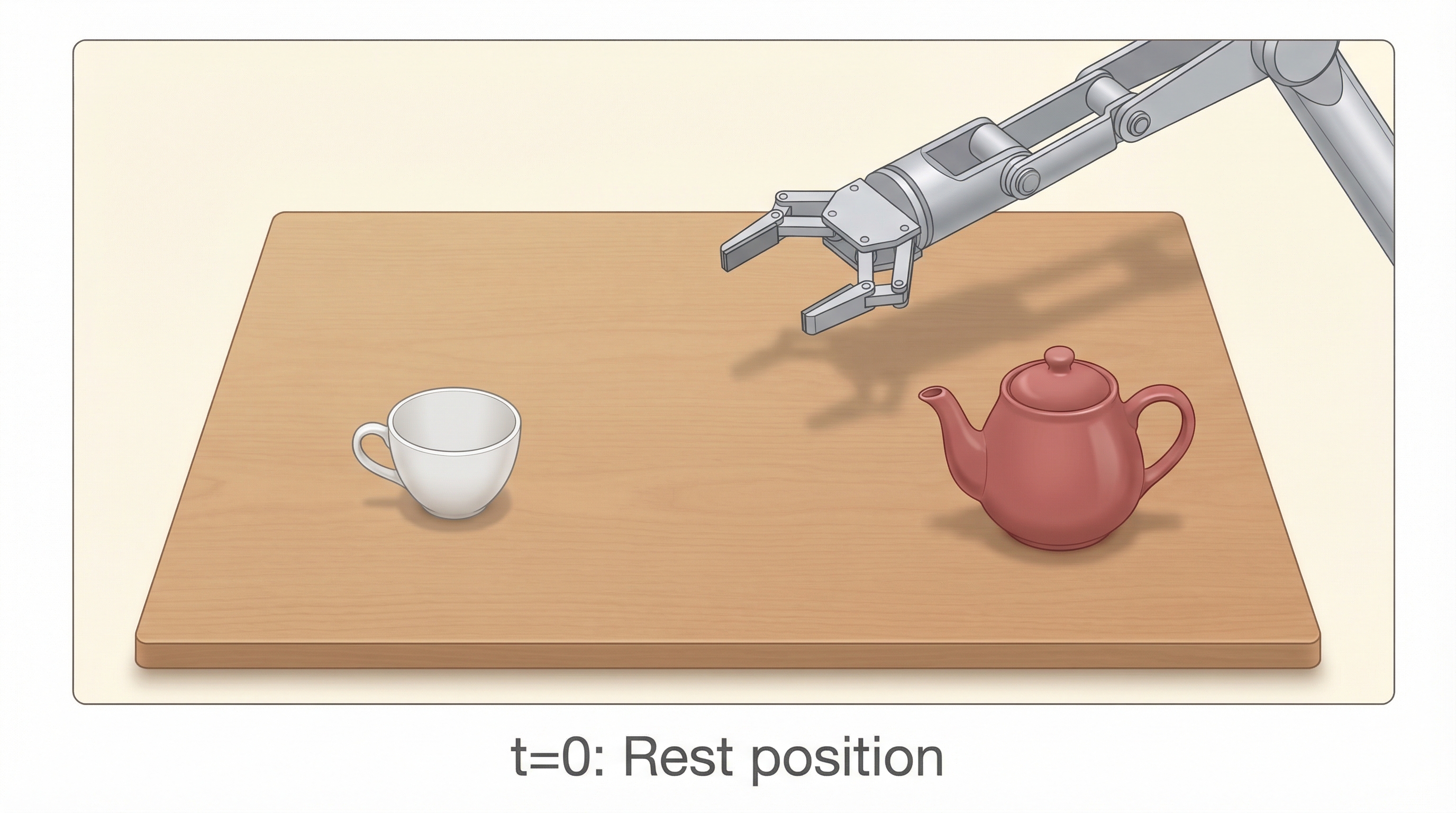
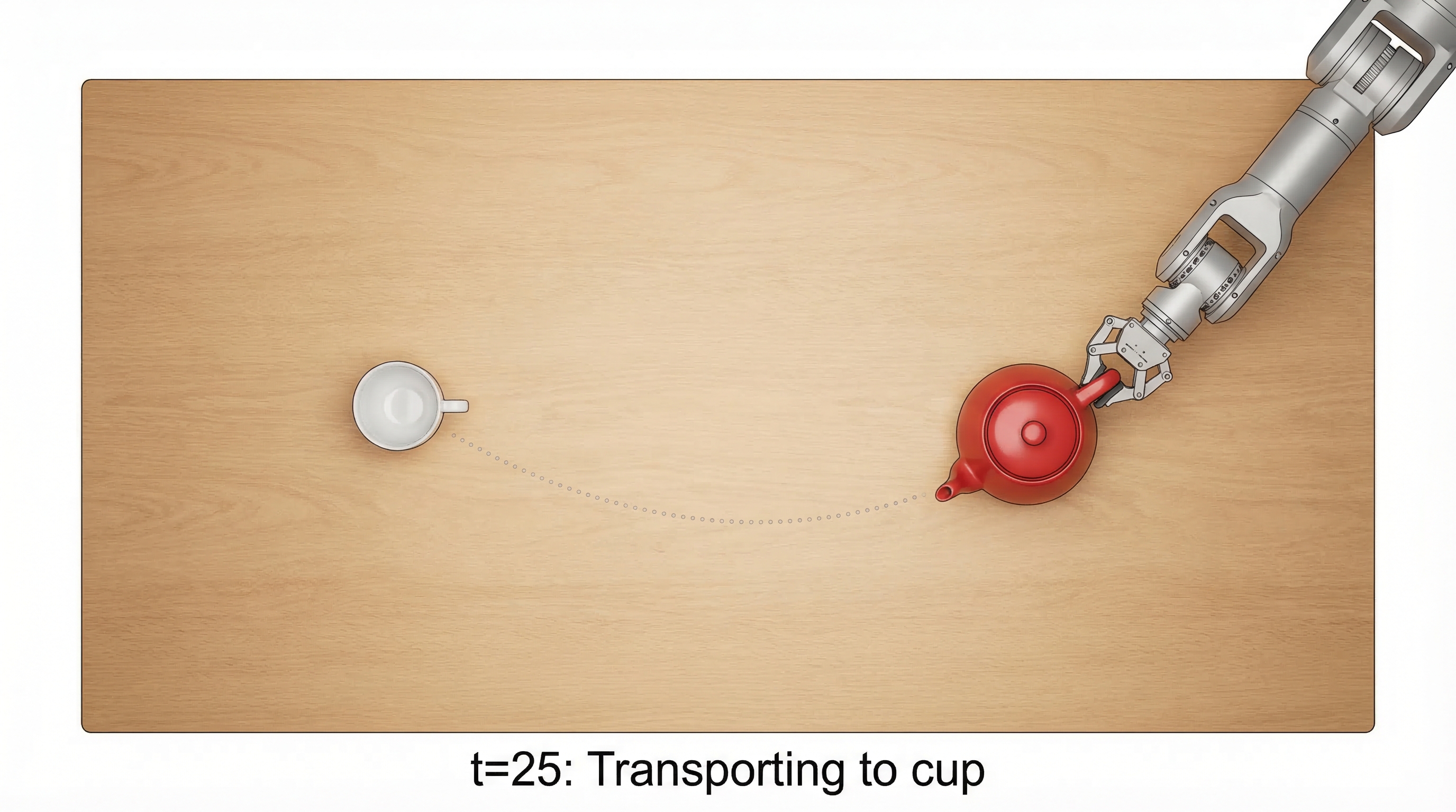
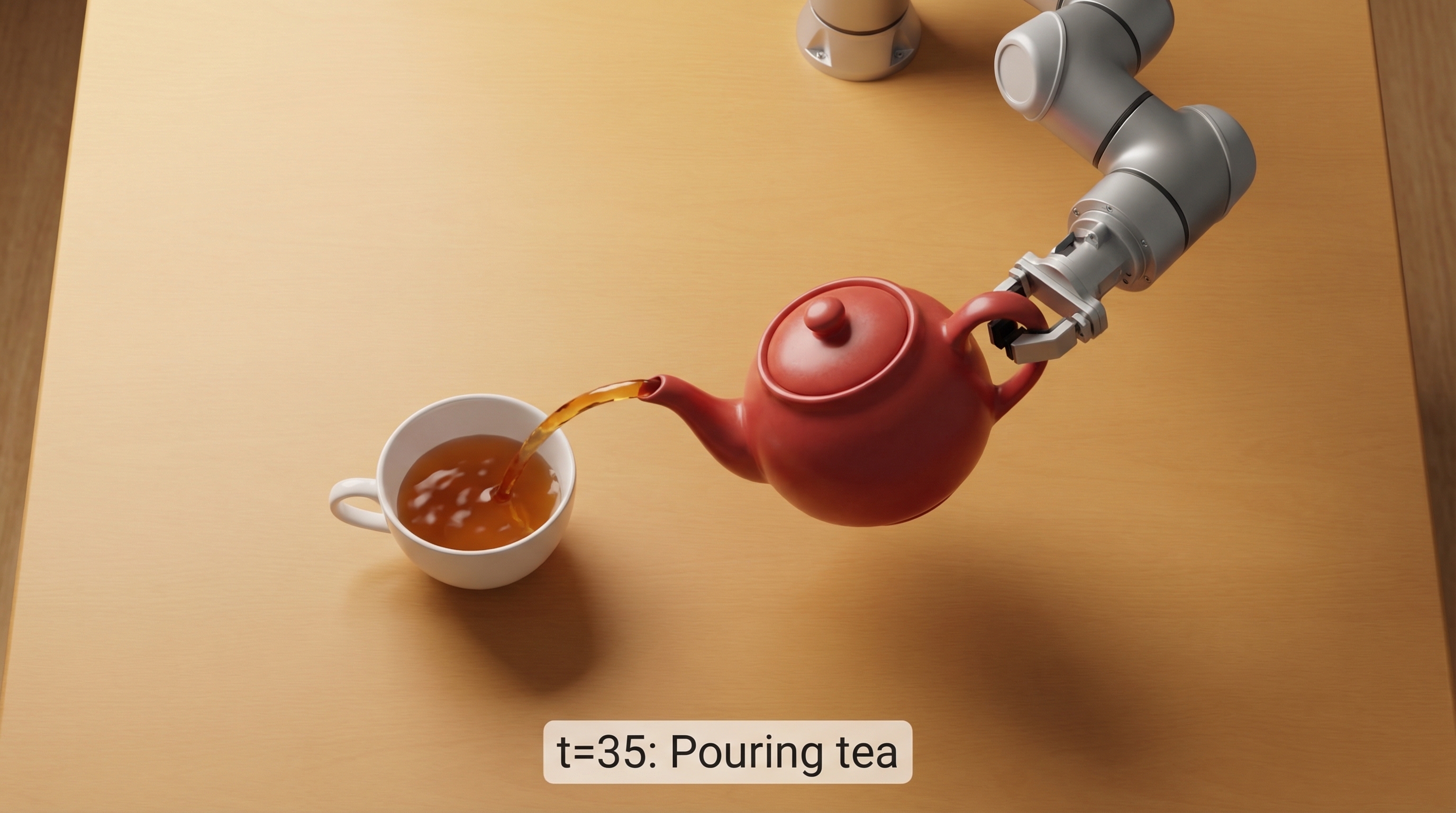
A 6-DOF robotic arm must pour tea from a teapot into a cup. We have 50 frames (5 seconds at 10 Hz) of expert demonstration data.
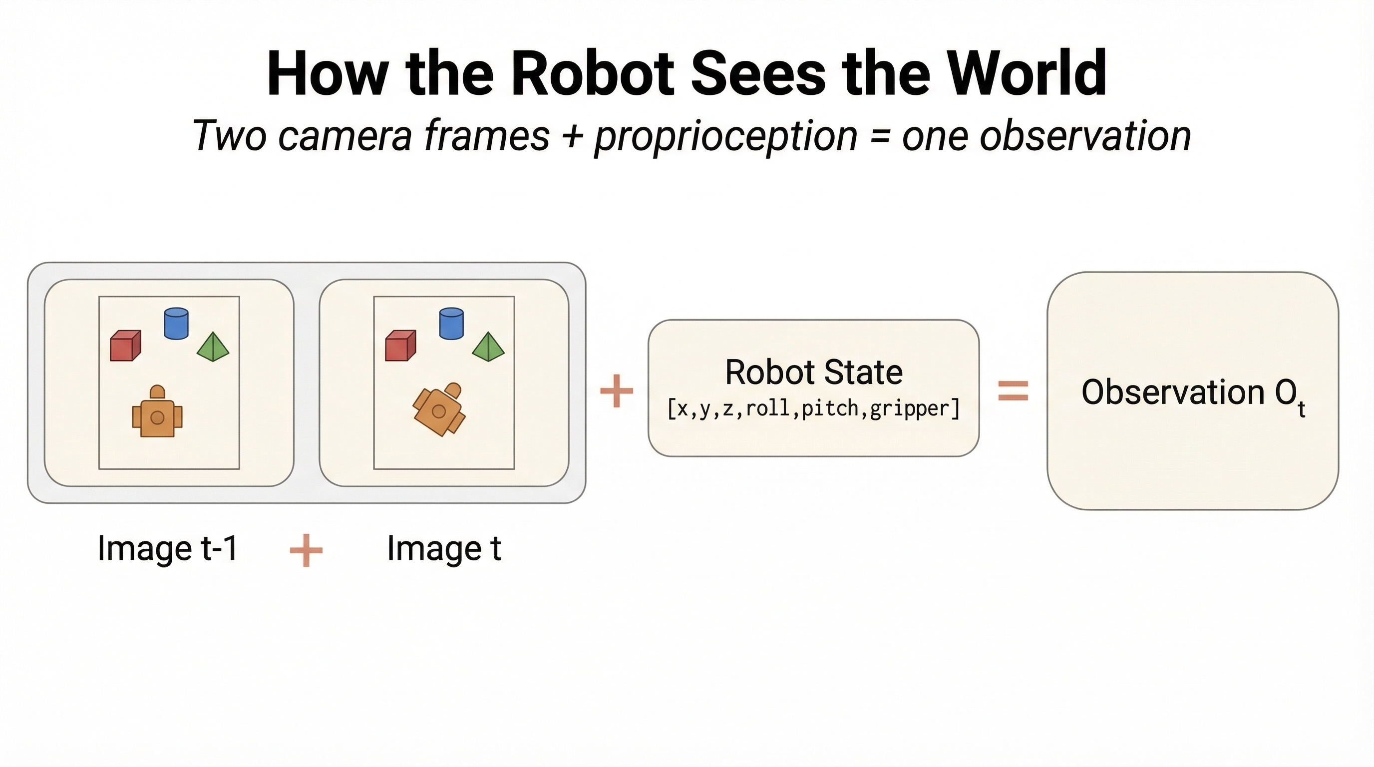
Each frame contains:
Top-down view showing teapot, cup, and robot arm
[x, y, z, roll, pitch, gripper] — joint positions
[Δx, Δy, Δz, Δroll, Δpitch, Δgripper] — target deltas
A human teleoperates the robot to pour tea. We record everything.
Scrub through the demonstration. The dots on the image show the gripper's next 16 planned waypoints — this is the action trajectory the diffusion model will learn to generate.
Camera observation with trajectory overlay
For each timestep t, we store a tuple:
The dataset has 50 such tuples for this one episode. In practice, we'd collect hundreds of episodes.
Each observation combines camera images with proprioceptive state.
The policy receives two consecutive camera frames (giving velocity information) plus the robot's joint state vector. Together, these form the observation that conditions the diffusion process.
Why two frames? A single snapshot shows position, but two frames reveal direction and speed — critical for smooth, reactive control.
Diffusion Policy uses three different time windows. This is the key concept.
Move the slider to change the "current timestep" and see how the three horizons shift.
The policy looks at the last 2 frames of observations. This gives it velocity information — not just where the robot is, but which direction it's moving.
The diffusion model outputs 16 action steps at once. Predicting more than we execute provides temporal consistency.
Of the 16 predicted actions, only the middle 8 are executed. Then we re-plan with fresh observations. This is receding-horizon control.
For a given current timestep t, we extract from the dataset:
The observation is the condition. The action trajectory is what gets noised and denoised.
The key insight: we corrupt the expert action trajectory with Gaussian noise.
The dots show the gripper's 16 planned waypoints (t through t+15). At k=0 the path is a smooth arc from teapot to cup. As k increases, each waypoint scatters — this is what noise does to the action trajectory.
Trajectory overlay on scene — noise jitters the path
6D action dimensions over time
Given a clean action trajectory A0, the forward process adds noise:
Here, āk goes from ~1 (clean) to ~0 (pure noise).
āk (cosine schedule) — how much signal remains at each step
This is where the neural network actually learns. Let's trace through one complete training step.
What happens over thousands of iterations.
Watch the loss decrease as the network trains. Each iteration samples a random batch, random timestep, random noise.
Training Loss (MSE between predicted and actual noise)
Iteration: 0
Loss: —
Sampled timestep k: —
Batch sample from frame: —
Press "Start Training" to begin.
After training, we reverse the diffusion process to generate actions from noise.
At k=100, the 16 waypoints are scattered randomly — the robot has no plan. As the network denoises, the waypoints converge into a smooth arc: the gripper's path from teapot to cup.
Trajectory denoising on scene image
Action dimensions converging to clean trajectory
After executing 8 actions, the robot captures new observations and runs inference again. This creates a closed-loop system.